Forecasting pipeline in R
R has a nice package support when it comes to forecasting. There is the forecast package which allows you to build several types of models:
- Arima – Autoregressive integrated moving average,
- Ets – Exponential smoothing state space model,
- Tbats – Exponential smoothing state space model with Box-Coxtransformation, ARMA errors, Trend and Seasonal components,
- Arfima – fractionally differenced Arima,
- Croston method
- Nnetar – Neural Network time series forecast
- Thetaf – Theta method forecast
and some more.
Additionally we can use forecastHybrid package for ensembling several models to improve forecast quality. For hierarchical time series we can leverage hts package. Very useful are also timetk package for time series creation and sweep package for tidying and simplified handling of forecast objects.
With those packages and some help from tidyverse we can build several forecasting models in a very convenient way.
HOW TO
Here I show how to create some more advanced forecasting in R, using the packages mentioned. I do not focus on data cleansing and preparation although this is an important part of every modelling. Instead I present how we can handle several time series simultaneously by doing data nesting, how to build model hybrids and how to perform yearly predictions using monthly data.
My example is based on bike_sales dataset from the sweep package.
|
1 2 3 4 5 6 7 8 9 10 |
library(tidyverse) library(lubridate) library(zoo) library(sweep) library(tidyr) library(forecast) library(forecastHybrid) library(timetk) head(bike_sales) |
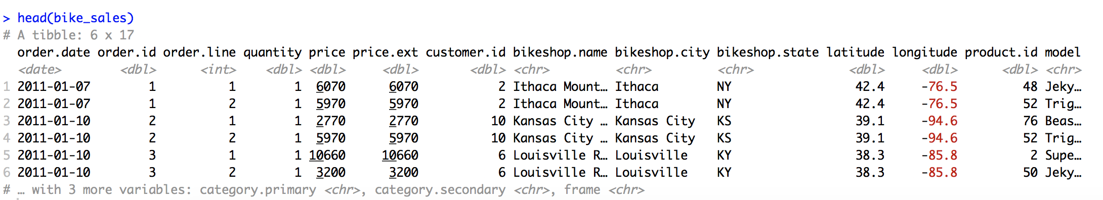
It is a fictional dataset, which contains bicycle orders over years 2011 to 2015. Results are stored with daily timestamps in 15644 rows and 17 columns. But I will use just three of them:
- order.date – holding forecasting timestamp
- category.secondary – specifying 9 different bike categories
- quantity – with number of purchased bikes
I want to forecast how many bikes were sold in years 2014 and 2015 and compare those with actuals.
Every bike category has assigned different number of daily data points. That is why first I aggregate the results to obtain monthly sale quantities.
|
1 2 3 4 |
data <- bike_sales %>% mutate(order.month = as_date(as.yearmon(order.date))) %>% group_by(category.secondary, order.month) %>% summarise(total.qty = sum(quantity)) |
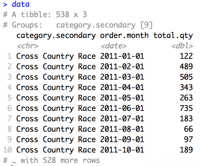
Now I have 60 data points for almost all categories.
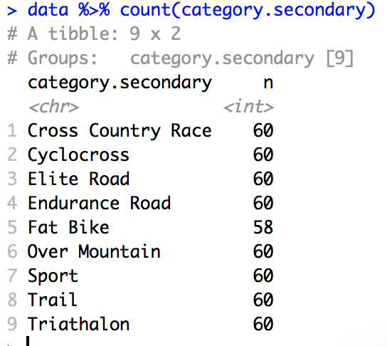
I have 9 bike categories and I want to perform separate forecast for each of those. To do that I use a technique called data nesting. It means combining all time-dependent variables into one structure per each category split.
|
1 2 3 4 |
nested_monthly <- data %>% group_by(category.secondary) %>% nest(.key = "series") %>% ungroup() |
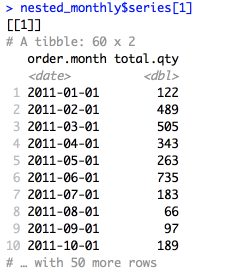
I ended up having just one data record per each of bike categories. In series column I have a list of nested tibbles, holding time variable and all values that are time dependent.
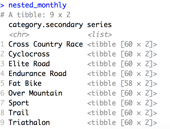
Each tibble has the same structure:
With such nested structure I can handle all 9 time series at the same time. I can build models for all bike categories simultaneously.
I want to perform two types of forecasts – monthly and yearly one. To get monthly results I perform classical forecast on monthly data. To obtain yearly figures, on the other hand, I use the technique described by Rob J. Hyndman for time preaggregations of the data. In principle I first replace current quantity values with sums of that many previous values as I have in aggregated time frame (so 12 last months for yearly results). On such preaggregates I then perform the modelling and forecasting. After that I just need to select proper results as our forecasts of interest (every 12th forecast would hold actual yearly values).
This method is better than simple results aggregation as it allows to easily determine confidence intervals of our predictions and gives good results overall.
Doing pure yearly forecast on yearly aggregates would not be possible on this dataset as there are only 5 years of data. That would mean building a model on 3 data points (2 for testing) which is not enough for any kind of forecasting.
For my two types of modelling I first create two types of time series – monthly ones and aggregated ones.
|
1 2 3 4 5 6 7 8 9 10 11 12 13 14 15 16 17 18 |
ts_data <- nested_monthly %>% mutate(train.ts = map(series, ~.x %>% filter(order.month < make_date(2014, 1, 1)) %>% tk_ts(frequency = 12, start = c(2011,1), end = c(2013,12), silent = T)), test.ts = map(series, ~.x %>% filter(order.month >= make_date(2014, 1, 1)) %>% tk_ts(frequency = 12, start = c(2014,1), end = c(2015,12), silent = T)), # aggregate results for yearly predictions train.ts.agg = map(train.ts, ~.x %>% stats::filter(., rep(1,12), sides = 1) %>% stats::window(start = c(2011, 12), end = c(2013, 12))), test.ts.agg = map(test.ts, ~.x %>% stats::filter(., rep(1,12), sides = 1) %>% stats::window(start = c(2014, 12), end = c(2015, 12)))) |
Training time series cover years 2011 – 2013 and testing years 2014 – 2015. map function comes to help with handling my nested tibbles. I create time series using tk_ts function and then preaggregate data with window function from stats package.
Now I can build models and do forecasts on both types of series. I use classical Arima model and a hybrid consisting of 4 models:
- Arima
- Tbats
- Ets
- Snaive
Hybrid is a model which we create by combining results of other models. We perform several predictions and then we weight the results of those to obtain one value per each time point. Hybrid models may give us better results than separate models as they can leverage different modelling techniques and combine them.
For building a model hybrid we may use as many models as we want, as long as we weight the results properly. Most typically we either use equal weights or weights inversely proportional to each models errors.
For hybrids I use forecastHybrid package.
|
1 2 3 4 5 6 7 8 9 10 11 12 13 14 15 16 17 |
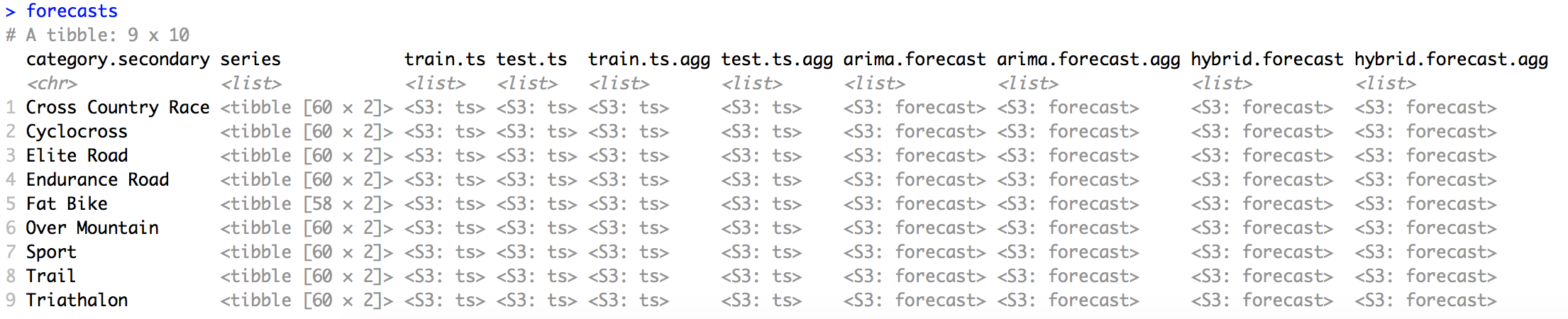
forecasts <- ts_data %>% mutate(arima.forecast = map(train.ts, ~.x %>% auto.arima(., stationary = F, seasonal = T, approximation = F) %>% forecast(., h = 24)), arima.forecast.agg = map(train.ts.agg, ~.x %>% auto.arima(., stationary = F, seasonal = T, approximation = F) %>% forecast(., h = 24)), hybrid.forecast = map(train.ts, ~.x %>% hybridModel(., models = "aetz", weights = "equal") %>% forecast(., h = 24)), hybrid.forecast.agg = map(train.ts.agg, ~.x %>% hybridModel(., models = "aetz", weights = "equal") %>% forecast(., h = 24))) |
hybridModel function can be provided with combination of several (at least two) models that we want to use and type of weights specifying way of combining the results .
In each forecast I specified 24 months for prediction. Finally I have 4 new columns holding results of different forecasts.
Now I need to select proper values as my yearly predictions.
|
1 2 3 4 5 6 7 8 9 10 11 12 13 14 15 16 |
forecasts_adj <- forecasts %>% mutate(arima.forecast.agg.fil = map(arima.forecast.agg, ~.x %>% sw_sweep(rename_index = "year") %>% filter(grepl("Dec", year)) %>% mutate(year = make_date(year(year), "01", "01")) %>% rename(total.qty = names(.)[3])), hybrid.forecast.agg.fil = map(hybrid.forecast.agg, ~.x %>% sw_sweep(rename_index = "year") %>% filter(grepl("Dec", year)) %>% mutate(year = make_date(year(year), "01", "01")) %>% rename(total.qty = names(.)[3])), test.ts.agg.fil = map(test.ts.agg, ~.x %>% tk_tbl(rename_index = "year") %>% filter(grepl("Dec", year)) %>% mutate(year = make_date(year(year), "01", "01")) %>% rename(total.qty = names(.)[2]))) |
I select results assigned to December of each year of interest. My forecasts look like this:


and aggregated ones:


Now let’s visualize the results with some plots.
|
1 2 3 4 5 6 7 8 9 10 11 12 13 14 15 16 17 18 19 20 21 22 23 24 25 26 27 28 29 30 31 32 33 34 35 36 37 38 39 40 41 42 43 44 45 46 47 48 49 50 51 52 53 54 55 56 57 58 59 |
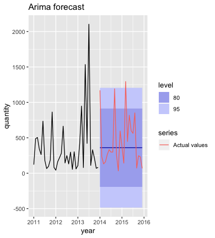
plots <- forecasts_adj %>% mutate(arima.plot = pmap(.l = list(af = arima.forecast, tts = test.ts), .f = function(af, tts){ af %>% autoplot() + autolayer(object = tts, series = "Actual values") + labs(title = "Arima forecast") + scale_y_continuous("quantity") + xlab("year")}), hybrid.plot = pmap(.l = list(af = hybrid.forecast, tts = test.ts), .f = function(af, tts){ af %>% autoplot() + autolayer(object = tts, series = "Actual values") + labs(title = "Hybrid forecast") + scale_y_continuous("quantity") + xlab("year")}), arima.agg.plot = pmap(.l = list(af = arima.forecast.agg.fil, tts = test.ts.agg.fil), .f = function(af, tts){ af %>% ggplot(aes(x = year, y = total.qty)) + geom_ribbon(aes(ymin = lo.95, ymax = hi.95), fill = "#D5DBFF", color = NA, size = 0) + geom_ribbon(aes(ymin = lo.80, ymax = hi.80, fill = key), fill = "#596DD5", color = NA, size = 0, alpha = 0.8) + geom_line(data = af, size = 1) + geom_line(data = tts, inherit.aes = T, colour = "red") + labs(title = "Arima aggregated forecast") + scale_y_continuous("quantity") + xlab("year")}), hybrid.agg.plot = pmap(.l = list(af = hybrid.forecast.agg.fil, tts = test.ts.agg.fil), .f = function(af, tts){ af %>% ggplot(aes(x = year, y = total.qty)) + geom_ribbon(aes(ymin = lo.95, ymax = hi.95), fill = "#D5DBFF", color = NA, size = 0) + geom_ribbon(aes(ymin = lo.80, ymax = hi.80, fill = key), fill = "#596DD5", color = NA, size = 0, alpha = 0.8) + geom_line(data = af, size = 1) + geom_line(data = tts, inherit.aes = T, colour = "red") + labs(title = "Hybrid aggregated forecast") + scale_y_continuous("quantity") + xlab("year")})) |
Here are monthly results:

And here yearly ones:
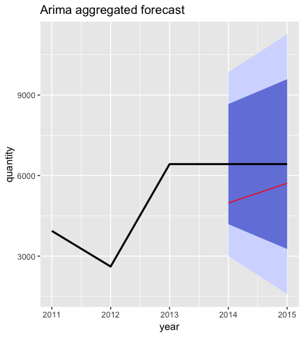

Of course yearly results are more smooth than monthly ones. We can also see that results of hybrid were better than ones obtained with Arima for Cross Country Race bikes.
With data nesting you can handle several time series all together. You can build different models for each series and even aggregate data on different levels. I find this data representation very useful for forecasting.
In many cases hybrid models perform better than single ones, but not always. It makes sense to combine several techniques if each of them performs ok for given data.
You can perform time aggregations on different levels (hourly data to daily, weekly to monthly…). I like particular method presented as it works nicely and allows to establish sensible confidence intervals for the forecasts.
Note: Currently fable package for tidy time series forecasting is being developed. This will most likely add some more tidy structure for constructing and handling time series.